A traditional way of shaping data in Excel is by using the VLOOKUP() function.  After identifying the item to look up and the array in which to search for it, a range is identified where the new information can be found.  The VLOOKUP() uses a vertical search of a data table.

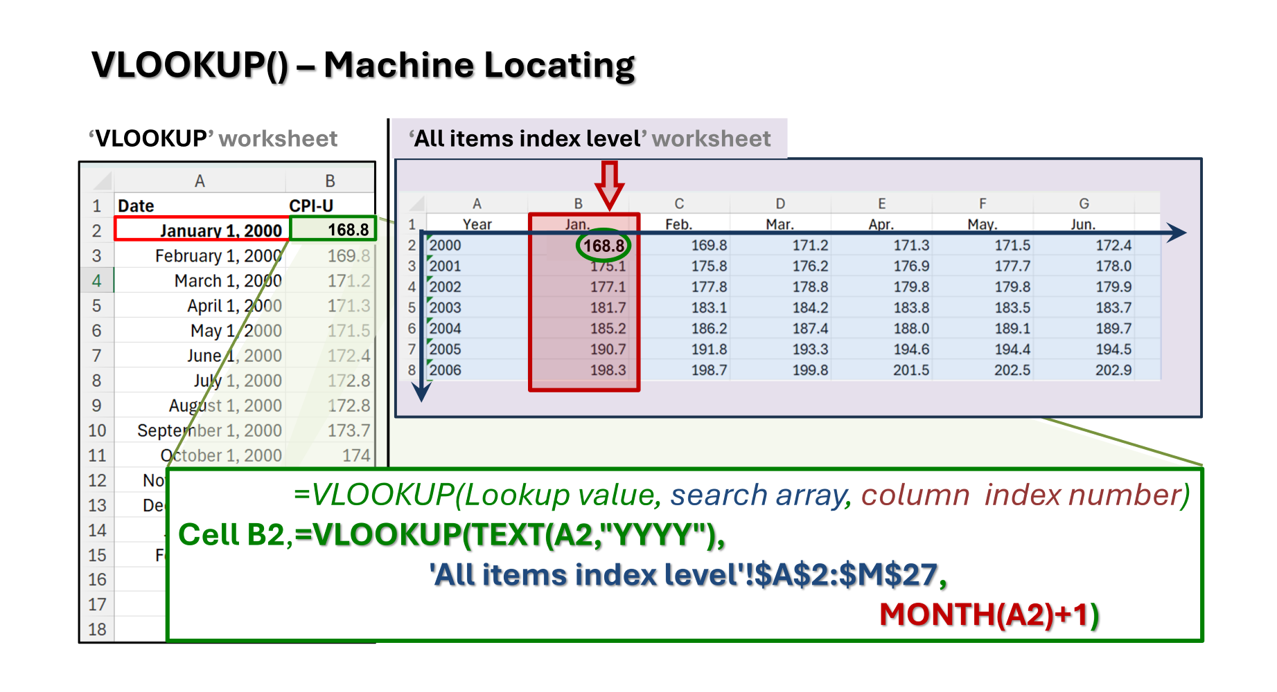
=VLOOKUP(Lookup value, search array, column index number)

There are other ‘flavors’ of lookup functions.  HLOOKUP() searches horizontally, and XLOOKUP(), uses range addresses to move beyond the more rigid search array structure of vertical or horizontal searches.  This post looks at VLOOKUP() for its simplicity of description and execution.

The problem and focus of these data shaping What the Function lessons, is that downloaded data may not arrive in the format desired for analysis.  After finding the necessary data, the available shape should not be the barrier for understanding.

The base dataset was downloaded from the Bureau of Labor and Statistics (BLS), Consumer Price Index (CPI).  This was covered in the blog post, Excel Data Shaping Fundamentals File Prep – What the Function.  There is a companion YouTube video that guides you through the steps at: https://youtu.be/M4agde_8zio.

The dates in the downloaded file are in a text format.  This is intuitive for the 3-character months (Jan, Feb, Mar,…), but less so for the row labels in the first column that are in years that look like number (2000, 2001, 2002,…).  Still they are saved as text, not values.

The options are to convert the downloaded dates to values, create text character dates in the newly shaped dataset, or create value-based dates in the new worksheet and convert them.  The pathway chosen for this lesson is the latter, to create numeric dates and convert them to text in the function syntax.

Starting in the file with the downloaded BLS, ‘All items index level’ worksheet table, add a new worksheet.  Then in Column A, add a Date label in row one.  In rows 2 through 4, add 1/1/2000, 2/1/2000, and 3/1/2000.  Highlight the three dates and hold the left-mouse button down on the little green box in the lower right corner of the highlighted range.  Drag it would to row 305 (4/1/2025) and release the mouse.  This fills the date range.

In Cell B2, enter the VLOOKUP() function.  The more specific formula required in Cell B2 is: Cell B2,=VLOOKUP(TEXT(A2,”YYYY”),’All items index level’!$A$2:$M$27,MONTH(A2)+1)

The formula above from the equal sign on the left to the parathesis on the right can be copied directly into Cell B2 of the new sheet, if everything has been done as has been described.

The TEXT() function grabs the year value from the numeric date in Cell A2 and delivers it for the search criteria as a text year – just like the text years in column A of the BLS CPI table.  The format code, “YYYY”, is for the 4-character year.

The ‘All items index level’!$A$2:$M$27, is the range for the search array.  This can be entered by clicking on the other worksheet, All items index level, and highlighting the table with all the columns and all the rows, except the first row of month headings.  The $-sign anchors need to be added before the A2:M27, column and row headings.  These can be typed in or added by clicking in each cell address and typing the F4 key.  This key toggles $-signs through each of the 4 configurations.

The last element of the VLOOKUP() function is the column number (within the search array).  This is done in the current formula using the MONTH() function.  This pulls the numeric month from the numeric date in Column A.  For January, it delivers a ‘1’.  For February, it delivers a ‘2’, and so on.  The only problem is that the January CPI values are in the second column of the search array.  The first column has the text dates in it.  But we can simply add the number, 1, to each monthly response and it will provide the correct column number.  The ‘+1’ does that after the month value.  This provide the correct monthly column number.

The last step is to copy the completed function instructions in Cell B2 to the rest of the table.  The most direct way to do this is using key stroke shortcuts.  From B2, move the active cell (green box) to Cell A2.  Then type, End, down arrow.  This moves the active cell from A2 to A305 (4/1/2025).  Right arrow the active cell to B305.  Then while holding the shift key down, type End, up arrow.  This will highlight all the cells between B305 and B2.  Right click and paste the formula into the highlighted range.

Check the last cell in row 305 with the April 2025 CPI value in the All items index level worksheet.  They should both be 320.795 (for April 2025 CPI-U).

Excel tasks discussed:

• VLOOKUP()
• TEXT()
• MONTH()
• Navigating table with End-arrow and Shift-End-arrow key combinations
• Filling dates by typing in 3 consecutive values and dragging lower right corner box to the endpoint.

Using VLOOKUP() to shift data in a spreadsheet is quick, fairly simple, and reliable.

The other two techniques, manual movement and INDEX/MATCH() functions can be found at:

1. Excel Data Shaping Fundamentals Cut and Paste – What the Function.  With the companion YouTube video at https://youtu.be/vgBFiA8b6h8 
2. Excel Data Shaping Fundamentals Index/Match – What the Function.  With the companion YouTube video at https://youtu.be/EfBLSrdWYio