One of the most powerful Excel function tools is the INDEX/MATCH() combination.  It can be set to find specific character strings and deliver the cell contents at the intersection of the row and column string matches.

This is the third post in the What the Function data transformation series.

1. Excel Data Shaping Fundamentals File Prep – What the Function.  This lesson outlined the challenge and listed common techniques for shaping data in Excel.  It also described steps in downloading the Bureau of Labor and Statistics (BLS), Consumer Price Index (CPI) as a base file for future post lessons.
2. Excel Data Shaping Fundamentals Cut and Paste – What the Function.  Cutting and pasting, or dragging and dropping, is not very sophisticated. That is where we all begin doing spreadsheet work. Still, even with more sophisticated tools in the data shaping toolbox, there is a place for manually pushing data around in a spreadsheet. The tradeoffs are increased risk of spreadsheet errors vs. simplicity of execution.

The INDEX/MATCH() function is at the opposite end of the nerd factor.  Solving real-time applied problems requires a suite of tools.  Focusing a post specifically on the INDEX/MATCH() function without other Excel hack distractions was not easy.  But with the companion video and this post, it should work.

The syntax of the two nested functions is defined as follows:

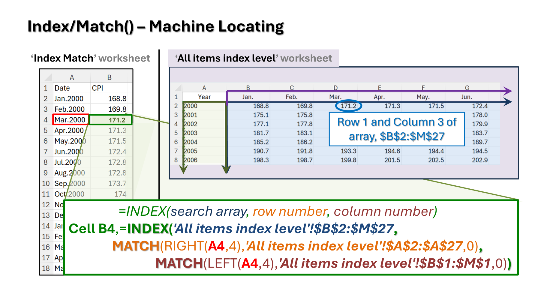
INDEX() = INDEX(search array, row number (within array), column number (within array)

MATCH() = MATCH(target value, range to search for target value, accuracy setting)

The key in this approach is to place the nested INDEX/MATCH() function in the cell where you want a certain result.

• The source worksheet, All items index level, is the name the BLS provided in the downloaded historical CPI data.
• The new data format takes place in a new sheet labeled, Index Match.
• The INDEX/MATCH() function is located in the Index Match worksheet transposing data located in the All items index level worksheet.  The formula in this post image represents the contents of Cell B4 in Row 4.  It uses the text date in Cell A4 to identify the dates for the corresponding CPI value, in this case March 2000.

Dates in Column A: The month and year references in the CPI downloaded data arrives are text strings that are not values.  They behave like words, even if they look like numbers.

In the Cut and Paste post, the dates were filled from January 2000 to April 2025 using the auto fill feature of Excel using three numeric dates for 1/1/2000, 2/1/2000, and 3/1/2000.  Once these three values were entered, it was possible to drag the highlighted dates to fill the entire column.

In this exercise, the new worksheet dates can be filled in as text values rather than numeric values.  Excel needs the entire 12 months of one year of text dates to autofill the other 25 years.  In Column A begin typing Jan.2000, Feb.2000, Mar.2000, etc., to Dec.2000.  With the first 12 months entered as text, these cells can be highlighted and dragged to the Apr.2025 row.

Entering the INDEX/MATCH() function: Starting in Cell B2 of the new, Index Match worksheet,

1. Enter the mandatory ‘=’ sign to begin an active formula.
2. As ‘Index(‘ is entered, Excel provides the syntax require below the active cell.
3. The first element, the search array, is in the BLS worksheet.  Select the All items index level worksheet and highlight everything but the column and row headings, or $B$2:$M$27 (The F4 key sets the ‘$’ sign anchors.  This can either be completed while entering the ranges or once all the ranges have been entered). Enter a comma, and the first element is complete.
4. The second INDEX() element is the row indicator.  This is where the MATCH() plays a role.  The MATCH() function has two elements: what to look for, and where to look for it.  This is the row indicator, so we are looking at ‘years’.  In the new sheet, the years are the second, or right-most 4-characters in Column A.  RIGHT(cell, # of characters) strips out the right 4 characters. Add a comma, then the second part is where to look.  In the original CPI worksheet this is Column A.  With your mouse, highlight the cells from $A$2:$A$27.  Add a comma, and then a final switch, which in this case is ‘0’.  This zero indicates only exact matches are desired.
5. The third INDEX() element is the column indicator.  This looks like the MATCH() function in the second element.  The two differences are directing the date lookup to the month component, or the left-most 4 characters in Column A.  LEFT(cell, # of characters completes that.  Add a comma and move on to highlight the where to look range.  For this element it is the column headings, or range $B$1:$M$1.  All the months in Row 1.  Also add a comma and the zero for exact matches only.  Add on end of parenthesis to end the MATCH function, then another parenthesis to close the INDEX function.

Easy peasy, right?  For Jan.2000, the CPI value displayed should be 168.8.

Before copying this formula to the rest of Column B, make sure that the three ranges from the All items index level have all the ‘$’ sign anchors.  These will not allow the ranges to change as copied.  The one active cell in the new worksheet is A2 for Jan.2000.  This needs to change as it is copied, so no dollar signs in this reference.

A quick key-stroke short cut to copy this formula from B2 to the rest of Column B is to use the End-Arrow keys.  Click on A2.  Type End-down arrow to move to the bottom of Column A. Click the right arrow once, to move to the last active cell of the new table in Column B.  Now, hold down the Shift key, while typing End-up arrow.  This will highlight the entire active column back to B2 where we began.  Right click and paste the B2 cell contents in the highlighted area.

Using the Downloaded file from BLS as it was provided, causes and error code to appear in all the May CPI cells (#N/A).  This is due to the fact that May is a complete month name and the BLS did not provide a period for the 3-character month abbreviation.  In the All items index level worksheet, click on the May label (Cell E1) and add a period.  This will make the error code disappear.

An alternative fix would have been to simply request LEFT(A2,3) in the third INDEX() function element.  This would have used the left-most 3 characters and not paid attention to the period for any of the months.

This INDEX/MATCH() function is a powerful tool.  Well done.

One parting note, the CPI values that are arranged in a time-series column as desired, are the results of active formulas using information in another worksheet.  If these values are transformed further, it is good practice to copy the values (cell results) into another location or on top of the existing CPI values using formulas.  Unforeseen problems will arise from adding more layers of transformation to information that is location dependent (original BLS worksheet).

Good work this was a lot to cover.  Topics covered in this post:

• INDEX()
• MATCH()
• LEFT()
• RIGHT()
• End-arrow key and Shift-End-Arrow keys to move around and for highlighting large areas of the worksheet.
• $-sign anchors to keep absolute cell references absolute.
• Auto fill with text character dates.

There is a companion YOUTUBE video located at. https://youtu.be/EfBLSrdWYio